Why Do Even Excellent Traders Go Broke? The Kelly Criterion and Position Sizing Risk
Why Do Even Excellent Traders Go Broke?
As I learned more about trading, I became more aware of the risks and how easily money can be lost.
There is a strange phenomenon in the world of investment. Traders with a win rate of 55%, meaning they win more often than they lose, somehow still go bankrupt. On the other hand, there are investors with the exact same win rate who steadily increase their assets. What is the difference?
The answer lies in “Position Sizing.” No matter how excellent your investment strategy is, if you mistake the amount you bet at one time, you will eventually lose your assets. Conversely, even with a mediocre win rate, proper money management can lead to long-term success.
In this article, I will explain the “Kelly Criterion,” discovered by John L. Kelly Jr. of Bell Labs in 1956, using Python simulations. This mathematical method teaches us the optimal bet size to increase assets most efficiently over the long term.
In a nutshell, Kelly Criterion tells us Given a small edge in win probability and odds, what fraction of your capital should you risk to maximize long term growth?
What you will learn in this article:
- The mathematical meaning and formula of the Kelly Criterion
- Why excessive betting leads to bankruptcy
- Verification through Python simulation
- Application to practical investment
All the code below can be found or downloaded here:
Basics of the Kelly Criterion: Understanding with a Simple Example
First, let’s consider a very simple betting game. You flip a coin; if it’s heads, your bet doubles (you win the bet amount). If it’s tails, you lose the entire bet amount. However, this is not a normal coin - it is a slightly favorable coin that lands on heads with a 55% probability.
You have 10K USD. When repeating this game 250 times, how much should you bet each time?
Intuitively, you might think, “If the win rate is 55%, I should bet a lot to make more money.” However, this is a big mistake. When we actually simulate it, surprising results become visible.
The Kelly Criterion Formula
The formula for the Kelly Criterion is as follows:
\[f^* = \frac{bp - q}{b}\]Where:
- f*: the optimal fraction of capital to bet
- p: win probability
- q = 1 − p: loss probability
- b: odds (here, 1 meaning you win 1x your bet)
Applying this to our example with a 55% win rate and 1:1 odds:
\[f^* = \frac{1 \times 0.55 - 0.45}{1} = 0.10\]In other words, the result is that betting 10% of your assets each time is optimal.
Important Point:
Even with a 55% win rate, the optimal bet rate is only 10%. This is a much more conservative value than intuition suggests.
Verifying with Python Simulation
Theory alone is hard to visualize, so let’s actually simulate it. The code below repeats the game thousands of times with different bet rates and visualizes the results.
Calculating the Kelly Fraction
def kelly_fraction(p: float, b: float = 1.0) -> float:
    """Function to calculate the Kelly fraction

    Args:
        p: Win probability
        b: Odds (Multiplier when winning - 1)

    Returns:
        Optimal bet fraction
    """
    q = 1.0 - p  # Loss probability
    return (b * p - q) / b
In this simulation, we perform 5,000 trials and track what results each bet rate brings. The important thing is not to use the average value, but the index called “Expected Logarithmic Growth Rate.”
Why use log growth?
In trading you care about compounding, not just the average win per bet. A common way to score that is expected log growth:
\[g(f) = p \log(1 + bf) + (1-p) \log(1 - f)\]The $f$ that maximizes this function is the Kelly fraction $f^*$.
What this simulation is really saying
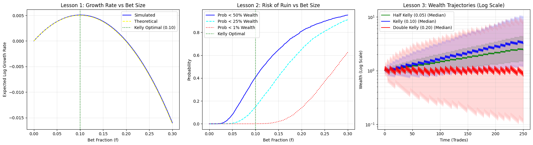 Kelly Criterion simulation results showing: (left) Expected logarithmic growth rate vs bet fraction, (middle) Drawdown probability for different thresholds, (right) Wealth evolution over time for Half Kelly, Kelly, and Double Kelly strategies.
Three takeaways:
- Kelly is the sweet spot: here it lands around $f \approx 0.10$.
- Going bigger hurts fast: push past that and growth drops; at double Kelly it can go negative.
- Big bets get ugly: drawdowns get more likely and the outcomes spread out a lot.
The right panel shows what that feels like under three bet sizes:
| Strategy | Bet Rate | Characteristics |
|---|---|---|
| Half Kelly | 0.05 | Very stable, but growth is slow |
| Kelly | 0.10 | Balanced and grows steadily |
| Double Kelly | 0.20 | Swings violently and often leads to capital decline |
The percentile bands (25th–75th) show how messy it gets when you size up too much.
Hands-on example: Kelly as implicit volatility targeting (AAPL and NVDA)
In practice people often use a mean-variance-ish version of Kelly. For a single asset, the leverage comes out like this:
\[L^* = \frac{\mu}{\sigma^2}\]Here, $\mu$ is the expected excess return and $\sigma$ is volatility, both annualized.
Recall the Sharpe ratio (ref):
\[\text{Sharpe} = \frac{\mu}{\sigma}\]If you lever an asset by $L^*$, the resulting portfolio volatility is roughly:
\[\sigma_{\text{portfolio}} \approx L^* \cdot \sigma = \frac{\mu}{\sigma}\]That equals the Sharpe ratio.
So what does this look like in code?
The example below pulls daily prices for AAPL and NVDA, estimates returns and volatility, computes $L^*$, and turns that into weights with a couple simple constraints.
Note: I used the 3-month Treasury bill (DTB3) as a rough risk-free rate. You can also just fix it or ignore it.
if __name__ == "__main__":
    result = kelly_vol_target(
        symbols=["AAPL", "NVDA"],
        start_time=datetime(2023, 1, 1, tzinfo=timezone.utc),
        end_time=datetime(2024, 12, 31, tzinfo=timezone.utc),
        series_id="DTB3",
    )
    print(result.round(4))
Output:
        mu_excess   sigma  kelly_L  weight
symbol
AAPL       0.2417  0.2268   4.6990  0.7000
NVDA       0.2035  1.0449   0.1864  0.0381
At first glance, both stocks appear attractive. Each has a strong estimated excess return, but their volatility profiles differ sharply. Because Kelly leverage scales with excess return divided by variance, volatility dominates the sizing decision.
Practical Application: Applying Theory to Real Investment
You understand the theory of the Kelly Criterion by now. However, to apply it to actual investment, there are several important considerations.
Practical caveats
- You don’t know the inputs: $\mu$ and $\sigma$ (or $p$ and $b$) are guesses. If your edge estimate is too rosy, full Kelly will have you taking way too much risk.
- What people do: fractional Kelly (half/quarter) and some hard caps (leverage, drawdown).
- Portfolios aren’t one bet: correlations matter, and “add up the single-asset Kelly sizes” can blow past 100% fast.
- What people do: put it in an optimizer with a risk budget and exposure limits.
- You still have to sleep at night: full Kelly can swing a lot, and real accounts have margin rules and risk limits.
- What people do: pick a volatility/drawdown you can live with and scale down.
Summary: What to Learn from the Kelly Criterion
I hope you understood that the Kelly Criterion shows a fundamental principle in investment, not just a calculation formula for bets.
Do not bet excessively even with an advantage.
Even mathematically proven optimal values are recommended to be halved in practice. This is a manifestation of a humble attitude recognizing uncertainty and human limitations.
Also, the importance of the balance between theory and practice. The Kelly Criterion is a beautiful theory, but instead of applying it blindly, it is necessary to adjust it appropriately considering your risk tolerance, estimation uncertainty, and market characteristics.
Appendix: Mathematical Background For Deeper Understanding
The mathematics behind the Kelly Criterion is closely related to Information Theory. In fact, Kelly’s original paper was written in the context of information transmission.
Maximizing the expected logarithmic growth rate is equivalent to maximizing Entropy. More precisely, the Kelly Criterion can be interpreted as optimizing the efficiency of converting information obtained from betting into asset growth.
Perspective of Risk-Adjusted Return
In modern investment theory, risk-adjusted returns such as the Sharpe Ratio are emphasized. The Kelly Criterion can be interpreted as the optimal strategy when assuming a Logarithmic Utility Function.
A logarithmic utility function represents a risk-averse investor. It mathematically expresses the sensation that the joy of doubling assets is smaller than the sadness of halving assets. In this sense, the Kelly Criterion is not just a mathematical optimization, but a practical method reflecting human psychology.
Enjoy Reading This Article?
Here are some more articles you might like to read next: